Let’s look at 10 of the most helpful formulas in Google Sheets that are designed to save you time.
Setting Up a Formula
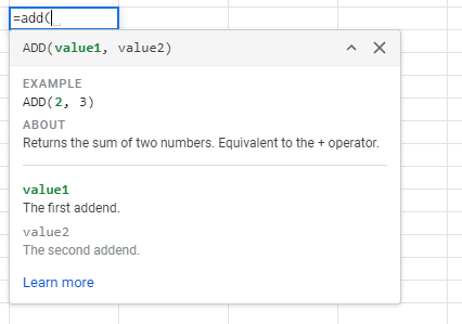
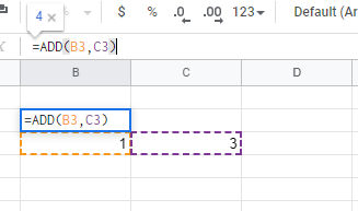
Using a formula on Google Sheets is easy. In a text box, just type “=” followed by the formula you want to use. There should be a little question mark box that pops up as you type a formula. Select that box to learn more about using that formula.For example, if we type in “=add(“ we’ll learn more about how to use this function. Sheets tells us that it returns the sum of two numbers and that we can format it by adding value 1, a comma, then value 2 within the parenthesis.That means that typing “=add(1,3)” should return the answer to 1+3.Instead of typing “1” and “3”, we can also refer to cells on Sheets. By adding the cell name (denoted by the column followed by the row), Sheets will automatically perform the formula for those given cells.So, if we type in “=add(B3,C3)”, the values from cells B3 and C3 will be added. It gives us the same answer. This approach works for most of the formulas in the following sections.
10 Helpful Formulas in Google Sheets to Save You Time
The following are 10 of the most helpful formulas in Google Sheets to save you time. There are plenty of hidden Sheets formulas that can help you, but these are ones that the everyday user can use and benefit from.
1. Ditch the Calendar with TODAY()
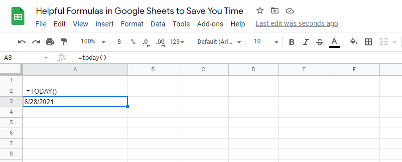
It feels like we catch ourselves asking “what’s today’s date?” every single day. In Sheets, it becomes an even bigger issue — tracking deadlines and counting down dates requires a daily update. That is, unless you use the TODAY() function.After putting it in a cell, you’re left with today’s date. It updates every day and doesn’t require you to do anything.Excel has a whole range of built-in date and time formulas. This makes it easy to find a difference between two dates. With the TODAY() function, you can have a constantly changing second variable.
2. COUNTIF() Makes Conditional Counting Easier
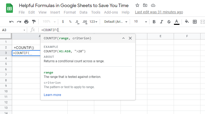
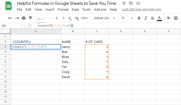
Sheets also lets you do a little bit of coding using what’s known as “conditional counting”. This is when you only count an item if it falls within certain criteria.For example, if you want to know how many of your survey participants own two or more cars, you can use a COUNTIF() statement. The condition would be a value that’s greater than or equal to two.Without using this formula, you would have to scan through the data by hand and find the number you’re looking for. There are other IF functions like this you can use as well such as SUMIF, AVERAGEIF, and more.
3. Add Cells with SUM()
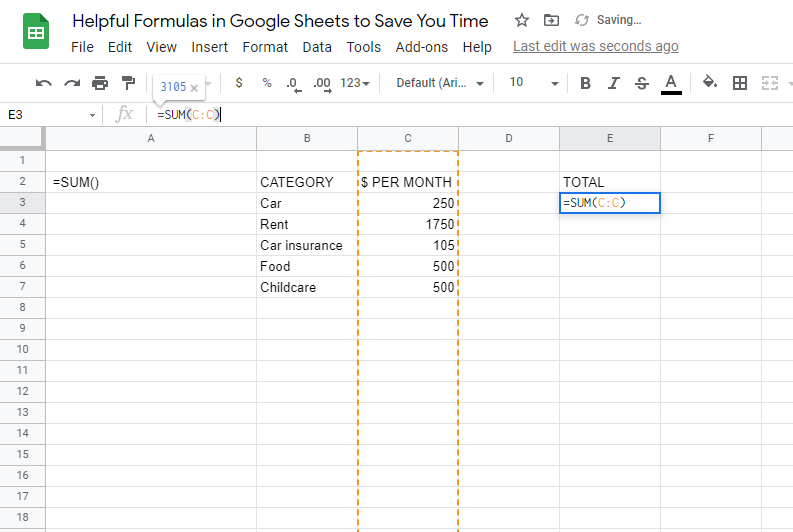
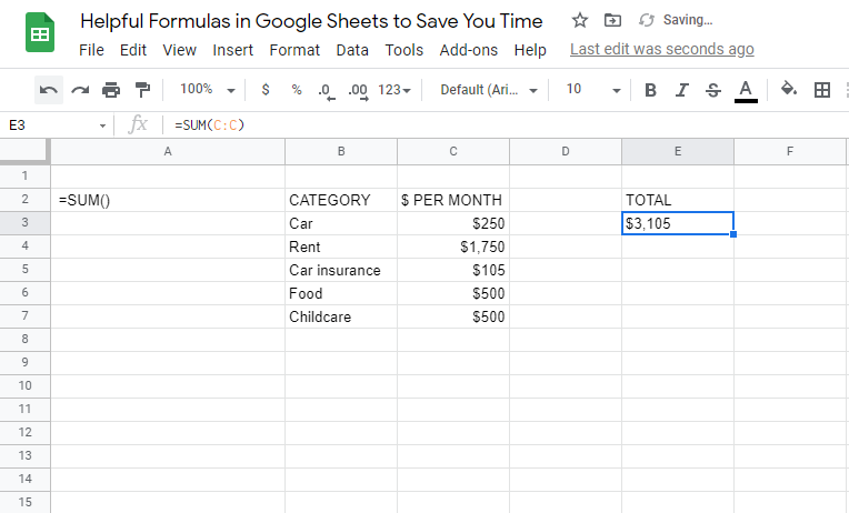
One of our favorite functions is the SUM() function. It adds together all the quantities within a selected range. A sum is just a bunch of numbers added together. For example, the sum of 2, 3, and 4 is 9.You can use SUM() to add a whole column together. As you keep adding new rows, the SUM() function will automatically update and add the new item. It can be used for positive, negative, or zero-value numbers.Want to make a quick budget? SUM() will be your best friend.
4. Put Text Together with CONCATENATE()
If you want to add strings of text together, you can’t just use addition. You’ll need to use a programming term called concatenation. This term refers to the idea of adding text together. You can concatenate multiple separate cells together and create a single cell that includes all of the text. Using CONCATENATE() is the automatic way of performing this process.Without this formula, you would have to copy and paste text separately into a single cell. This process takes a lot of time when you’re looking at files that contain multiple rows.This formula is great if you want to combine people’s first and last names or create personalized messages.
5. TRIM() Removes Unwanted Extra Spaces
Whenever blocks of text are copied and pasted from other sources, formatting becomes a nightmare. Many times, you’ll have unwanted spaces that ruin the overall format.You can either manually delete every space, or you can use the TRIM() command in Google Sheets. This command reduces the number of spaces in a message and leaves you with only one space between words.This could also be helpful for Sheets that are set up to accept written responses from users. It removes the human error of double-spacing by accident and results in a document that looks really clean.
6. TEXT() Converts Values to Other Formats
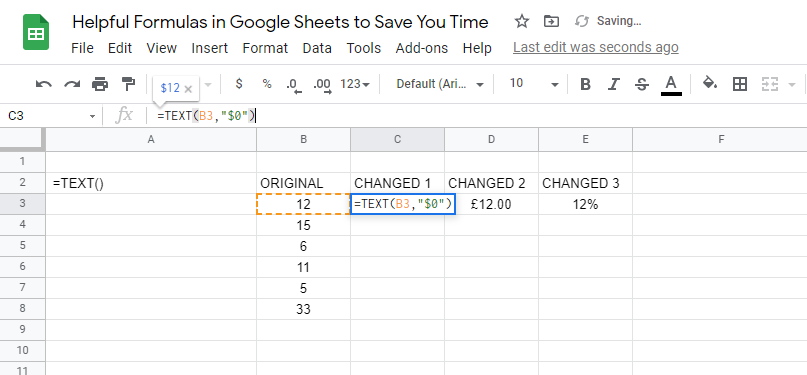
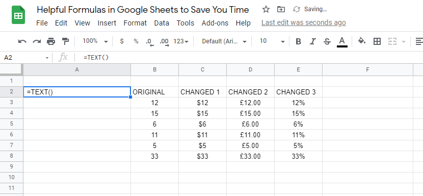
One of the big headaches in Google Sheets is reformatting values that are put into a cell. Sheets will try to guess which format you want, but you could be left changing a whole section of cells.Alternatively, you can try the TEXT() function. This formula will change the formatting from general text, strings of words, values, dollar amounts, percentages, dates, and a number of other options.If you’re copying and pasting a chunk of data that you need to turn into dollar values, for example, you can use this formula to do it. You can also change the number of decimals shown after the value.
7. Built-In Translation with GOOGLETRANSLATE()
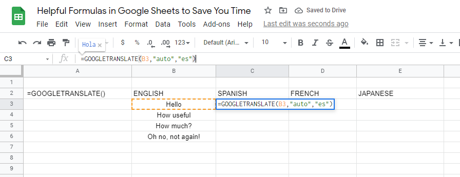
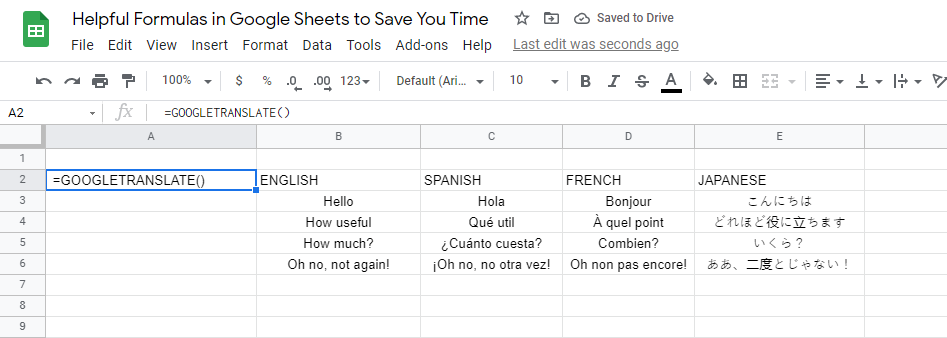
Sheets can also expedite your translations. If you have a column of phrases in a language you know, you can create multiple columns of a translated phrase into different languages.For example, we can translate common phrases from English to Spanish, French, and Japanese in a single document. This can help an international team understand the same document.This formula is courtesy of Google’s translation services. You can also use this formula to find out what language a certain text is by copying and pasting it into Sheets. You can keep the source language as “auto”, and Sheets will determine what language it is, then translate it into the selected language you can understand.
8. Quickly SORT() Data
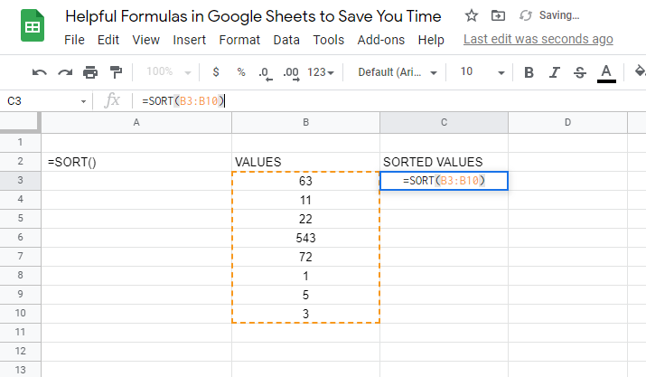
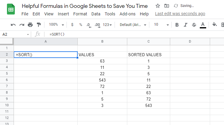
Maintaining a sorted list of data can be a headache. As new data is inputted or data is changed, your hand-sorted list will get disrupted.Rather than manually sorting the data every time it’s inserted, you can use the built-in SORT() command. This automatically generates a list of ascending or descending values. After running, it compiles the sorted list in its own row or column. You can then use this range to take additional steps in your Sheet.
9. Swap Rows and Columns with TRANSPOSE()
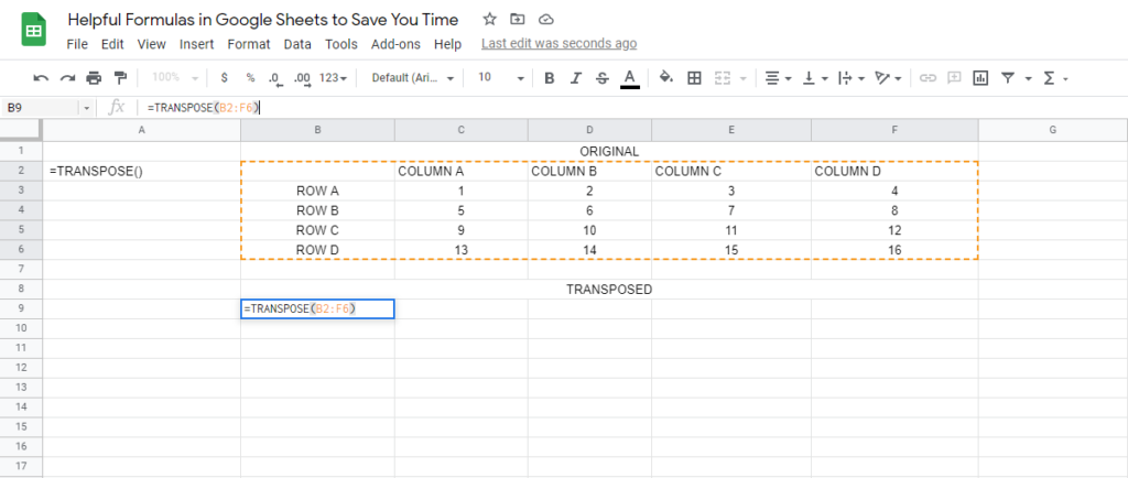
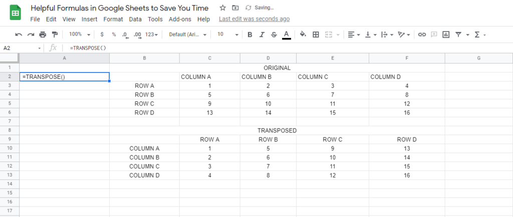
Did you accidentally swap the row and column of your sheet when you were first making it? Or maybe a client sent you over data that you’d like to add to your document, but the rows and columns need to be switched.Whatever the case, you can try the TRANSPOSE() command.Here’s how it works: The rows and columns are flipped around. The corresponding data in the table is also changed to ensure it’s in the correct place after the flip.As the old data is changed, the transposed table also updates and changes.
10. Quickly Find the AVERAGE()
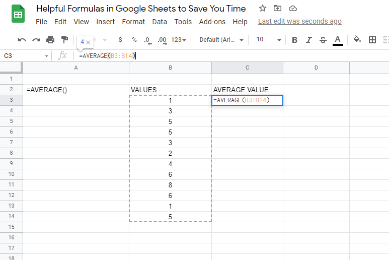
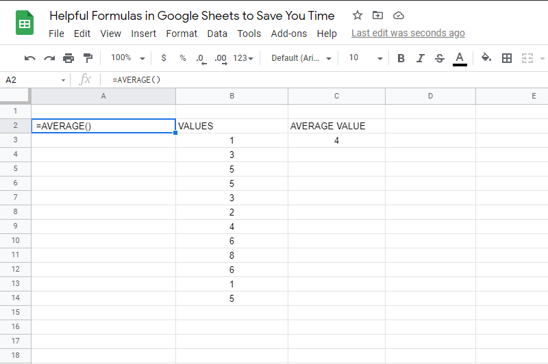
Using the AVERAGE() command in Sheets will spit out the mean of a given set of numbers. If you don’t remember, the average is when you add up all the numbers and divide by how many numbers there are.This is a useful math command. Without the AVERAGE() formula, you’ll be left solving it with paper and a calculator.Just select the range of numbers you want to find an average for, then Sheets will do the rest.
Use Formulas to Improve Your Google Sheets Efficiency
Time to open Sheets and try out these 10 helpful formulas you just learned. They’re designed to save you time and make your life easier. Try them out on your own and see how easy they are.Have a favorite formula that we missed? Leave a comment and let us know.
