In Excel, you can create filters on columns that will hide rows that do not match your filter. In addition, you can also use special functions in Excel to summarize data using only the filtered data.In this article, I’ll walk you through the steps for creating filters in Excel and also using built-in functions to summarize that filtered data.
Create Simple Filters in Excel
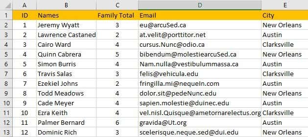
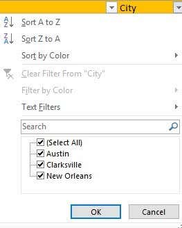
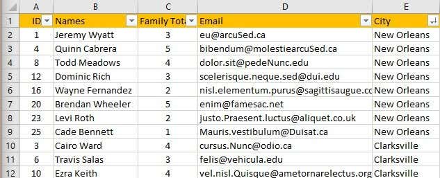
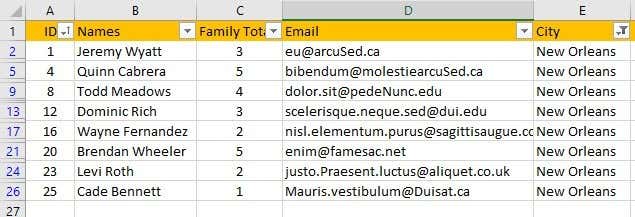
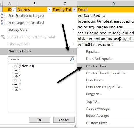
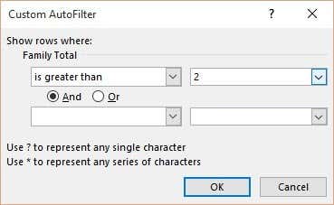
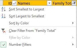
In Excel, you can create simple filters and complex filters. Let’s start off with simple filters. When working with filters, you should always have one row at the top that is used for labels. It’s not a requirement to have this row, but it makes working with filters a bit easier.Above, I have some fake data and I want to create a filter on the City column. In Excel, this is really easy to do. Go ahead and click on the Data tab in the ribbon and then click on the Filter button. You don’t have to select the data on the sheet or click in the first row either.When you click on Filter, each column in the first row will automatically have a small dropdown button added at the very right.Now go ahead and click on the dropdown arrow in the City column. You’ll see a couple of different options, which I will explain below.At the top, you can quickly sort all the rows by the values in the City column. Note that when you sort the data, it will move the entire row, not just the values in the City column. This will ensure that your data remains intact just as it was before.Also, it’s a good idea to add a column at the very front called ID and number it from one to however many rows you have in your worksheet. This way, you can always sort by the ID column and get your data back in the same order it was originally, if that is important to you.As you can see, all the data in the spreadsheet is now sorted based on the values in the City column. So far, no rows are hidden. Now let’s take a look at the checkboxes at the bottom of filter dialog. In my example, I have only three unique values in the City column and those three show up in the list.I went ahead and unchecked two cities and left one checked. Now I only have 8 rows of data showing and the rest are hidden. You can easily tell you are looking at filtered data if you check the row numbers at the far left. Depending on how many rows are hidden, you’ll see a few extra horizontal lines and the color of the numbers will be blue.Now let’s say I want to filter on a second column to further reduce the number of results. In column C, I have the total number of members in each family and I want to only see the results for families with more than two members.Go ahead and click on the dropdown arrow in Column C and you’ll see the same checkboxes for each unique value in the column. However, in this case, we want to click on Number Filters and then click on Greater Than. As you can see, there are a bunch of other options too.A new dialog will pop up and here you can type in the value for the filter. You can also add more than one criteria with an AND or OR function. You could say you want rows where the value is greater than 2 and not equal to 5, for example.Now I’m down to just 5 rows of data: families only from New Orleans and with 3 or more members. Easy enough? Note that you can easily clear a filter on a column by clicking on the dropdown and then clicking the Clear Filter From “Column Name” link.So that’s about it for simple filters in Excel. They are very easy to use and the results are pretty straight-forward. Now let’s take a look at complex filters using the Advanced filters dialog.
Create Advanced Filters in Excel
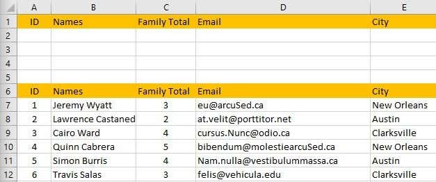
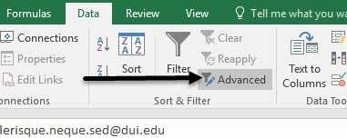
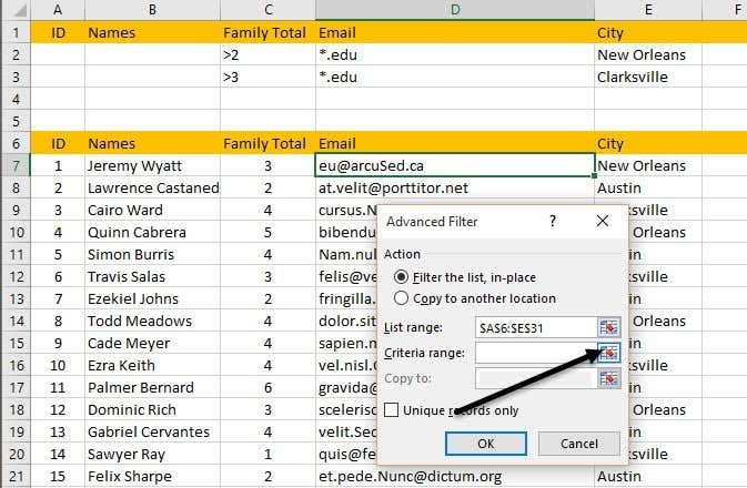
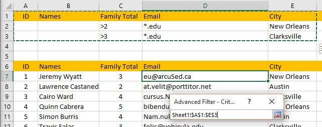
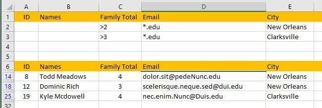
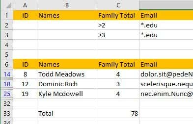
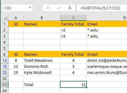
If you want to create more advanced filters, you have to use the Advanced filter dialog. For example, let’s say I wanted to see all families that live in New Orleans with more than 2 members in their family OR all families in Clarksville with more than 3 members in their family AND only the ones with a .EDU ending email address. Now you can’t do that with a simple filter.To do this, we need to setup the Excel sheet a little differently. Go ahead and insert a couple of rows above your set of data and copy the heading labels exactly into the first row like shown below.Now here is how advanced filters work. You have to first type your criteria into the columns at the top and then click the Advanced button under Sort & Filter on the Data tab.So what exactly can we type into those cells? OK, so let’s start with our example. We only want to see data from New Orleans or Clarksville, so let’s type those into cells E2 and E3.When you type values on different rows, it means OR. Now we want New Orleans families with more than two members and Clarksville families with more than 3 members. To do this, type in >2 in C2 and >3 in C3.Since >2 and New Orleans are on the same row, it will be an AND operator. The same is true for row 3 above. Finally, we want only the families with .EDU ending email address. To do this, just type in *.edu into both D2 and D3. The * symbol means any number of characters.Once you do that, click anywhere in your dataset and then click on the Advanced button. The List Range field will automatically figure out your dataset since you clicked into it before clicking the Advanced button. Now click on the small little button at the right of the Criteria range button.Select everything from A1 to E3 and then click on the same button again to get back to the Advanced Filter dialog. Click OK and your data should now be filtered!As you can see, now I have only 3 results that match all of those criteria. Note that the labels for the criteria range have to match exactly with the labels for the dataset in order for this to work.You can obviously create a lot more complicated queries using this method, so play around with it to get your desired results. Finally, let’s talk about applying summation functions to filtered data.
Summarizing Filtered Data
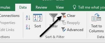
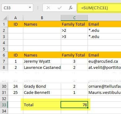
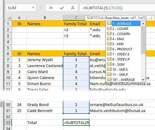
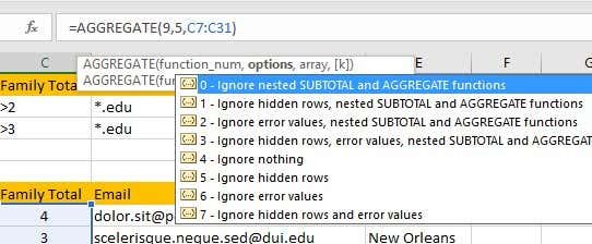
Now let’s say I want to sum up the number of family members on my filtered data, how would I got about doing that? Well, let’s clear our filter by clicking on the Clear button in the ribbon. Don’t worry, it’s very easy to apply the advanced filter again by simply clicking on the Advanced button and clicking OK again.At the bottom of our dataset, let’s add a cell called Total and then add a sum function to sum up the total family members. In my example, I just typed =SUM(C7:C31).So if I look at all families, I have 78 members total. Now let’s go ahead and reapply our Advanced filter and see what happens.Whoops! Instead of showing the correct number, 11, I still see the total is 78! Why is that? Well, the SUM function does not ignore hidden rows, so it is still doing the calculation using all the rows. Luckily, there are a couple of functions you can use to ignore hidden rows.The first is SUBTOTAL. Before we use any of these special functions, you will want to clear your filter and then type in the function.Once the filter is cleared, go ahead and type in =SUBTOTAL( and you should see a dropdown box appear with a bunch of options. Using this function, you first pick the type of summation function you want to use using a number.In our example, I want to use SUM, so I would type in the number 9 or just click on it from the dropdown. Then type a comma and select the range of cells.When you press enter, you should see the value of 78 is the same as previously. However, if you now apply the filter again, we will see 11!Excellent! That’s exactly what we want. Now you can adjust your filters and the value will always reflect only the rows that are currently showing.The second function that works pretty much exactly the same as the SUBTOTAL function is AGGREGATE. The only difference is that there is another parameter in the AGGREGATE function where you have to specify that you want to ignore hidden rows.The first parameter is the summation function you want to use and as with SUBTOTAL, 9 represents the SUM function. The second option is where you have to type in 5 to ignore hidden rows. The last parameter is the same and is the range of cells.You can also read my article on summary functions to learn how to use the AGGREGATE function and other functions like MODE, MEDIAN, AVERAGE, etc. in more detail.Hopefully, this article gives you a good starting point for creating and using filters in Excel. If you have any questions, feel free to post a comment. Enjoy!
