You can pull the items for your dropdown list from another range of cells, or you can enter them directly. Learn how to do both, as well as how to modify an existing dropdown list.
Create Manual Dropdown Lists in Google Sheets
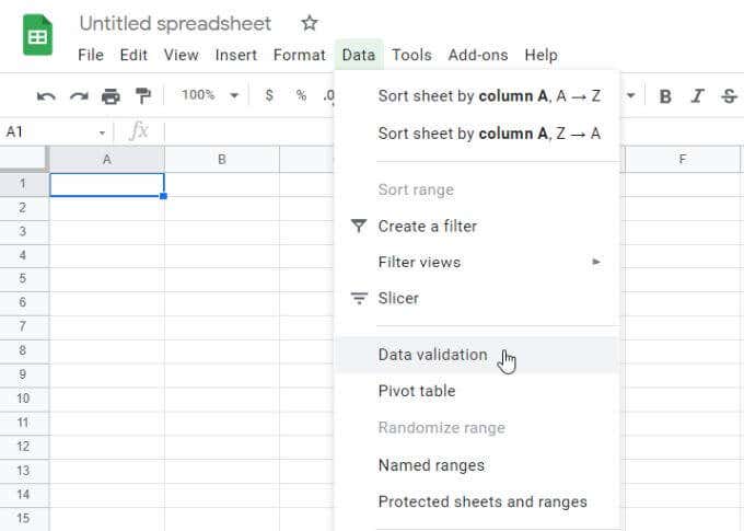
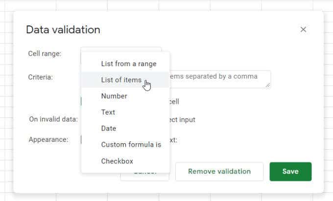
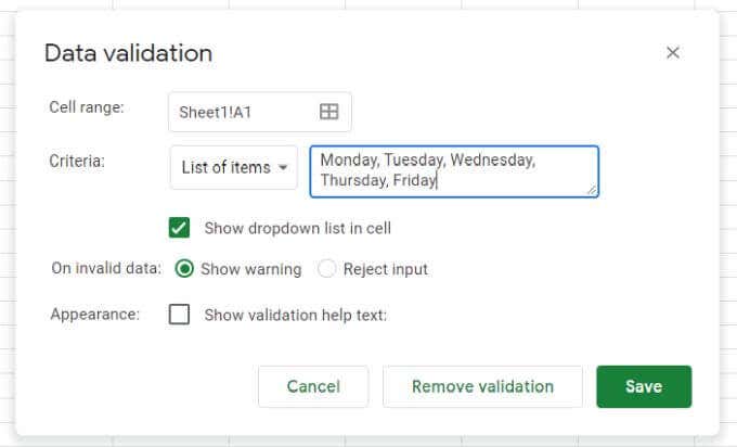
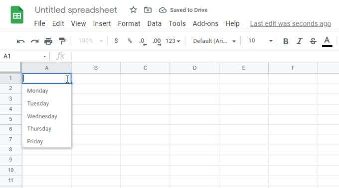
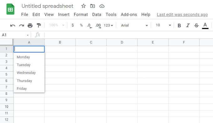
The fastest way to create a Google Sheets dropdown list is by listing the items inside the data validation settings.To do this:1. Select the cell where you want to create a dropdown list. Select Data from the menu, and then select Data validation.2. Next to Criteria, select List of items. 3. In the field next to this selection, type out the items you want to include in the dropdown list, separated by commas.4. Select the Save button, and you’ll see that the cell you selected now has a dropdown list.
Data Validation Options
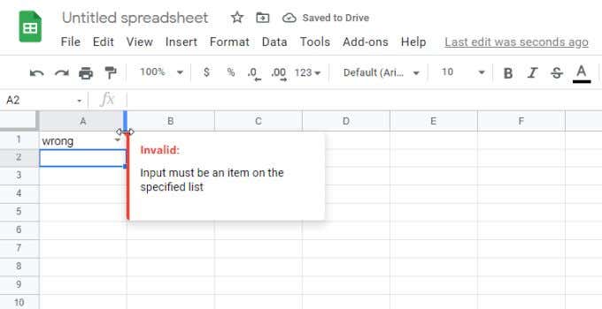
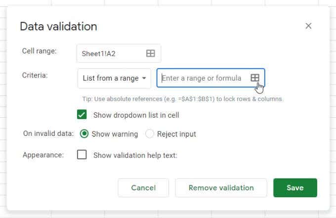
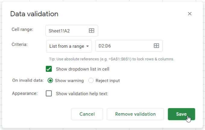
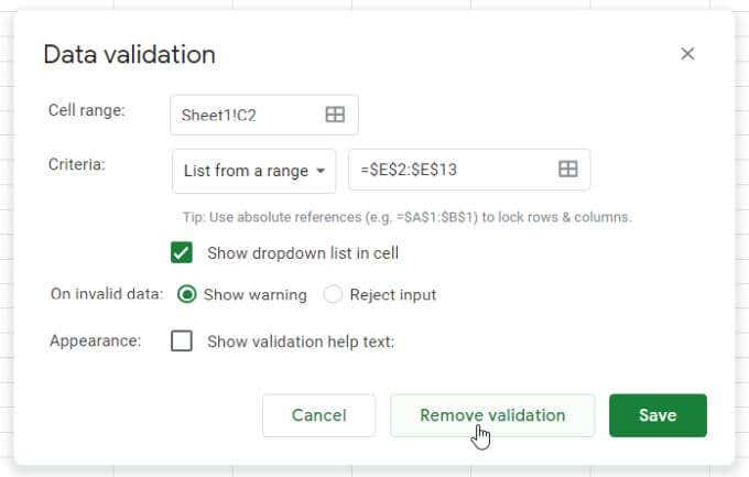
There are a few important settings in the Data validation window to note.If you deselect Show dropdown list in cell, the dropdown arrow will not appear. However, when the user starts typing, the list items will appear.In the On invalid data section, if you select Show warning, a red warning indicator will appear. This displays a message warning the user that the typed item doesn’t match anything in the list.If you select Reject input instead, Google Sheets will reject the entry and replace it with the first item of the dropdown list instead.In the Appearance section, if you select Show validation help text and type text into the field below it, that text will appear when the user selects the dropdown cell.
Create Dropdown Lists from a Google Sheets Range
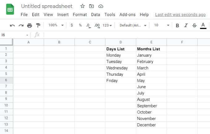
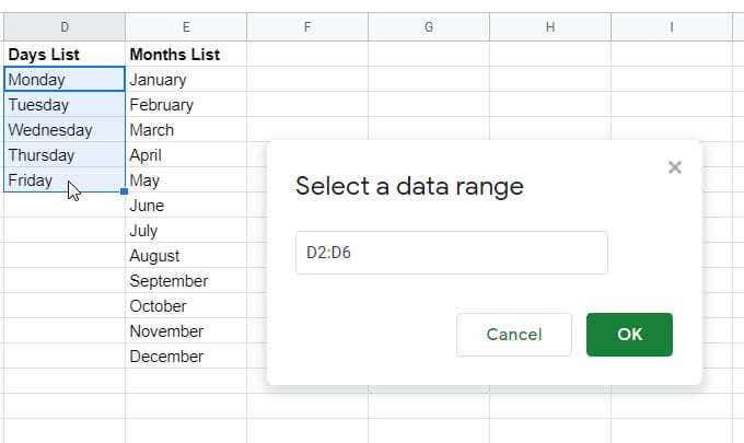
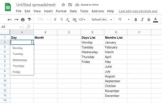
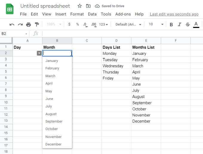
A more dynamic way to create Google Sheets dropdown lists is to use the contents of a range of cells to fill the list.To do this:1. First, create your validation lists in any range of cells. These don’t have to be in the same spreadsheet. You can create and select these lists in other spreadsheet tabs as well.2. Next, select the cell where you want to create a dropdown list. Select Data from the menu, and then select Data validation.3. This time, select List from a range from the Criteria dropdown list. Then, select the small grid selection icon to open the range selection window.4. Select the range you want to use as your list, and you’ll see the range text appear in the Select a data range field.5. Select OK to close out the selection window and return to the validation window. Configure the rest of the dropdown options you’d like and then select the Save button to finish.6. Now, you’ll see the range data appear as the dropdown list items in the cell you selected.7. Continue this same process for any other columns you’d like to add as a dynamic dropdown list.Using ranges as the source of your data is a great way to keep your spreadsheets updated without having to manually go through and update every dropdown list you’ve created.
Interesting Facts About Google Sheets Dropdown Lists
Google Sheets dropdown lists connected to ranges are the most useful because they dramatically reduce the overall maintenance of your spreadsheet.
Update Multiple Cells with One Range Change
This is especially true if you have many cells drawing data from a single range of items. If you want to update or change those list items, you’ll only have to make the change in a single range.Even if there are hundreds of cells with those list items, updating the range once will update all of those dropdown cells instantly.
Copying Validated Cells to Save Time
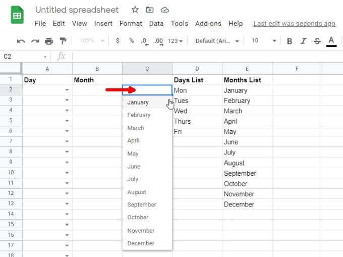
You can also save time by copying validated dropdown cells to any other cells. This saves the time of having to step through the process of stepping through the validation screens again.Copying validated cells is especially useful for selection lists like days, months, time, and other standard datasets.
Quickly Remove Cell Validation
Suppose you don’t want the list items included with any cell. You can quickly remove them by right-clicking the cell, selecting Validation, and then selecting Remove validation in the Data validation window.You’ll see the dropdown arrow disappear from the cell, and all of the dropdown items disappear. The cell will become just another normal spreadsheet cell.
Using Double Dropdown Lists in Google Sheets
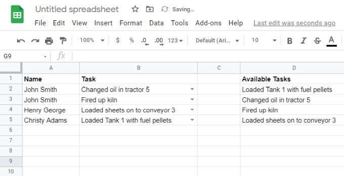
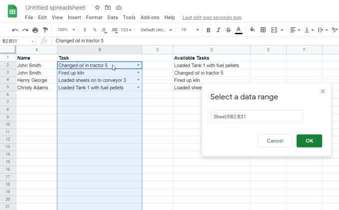
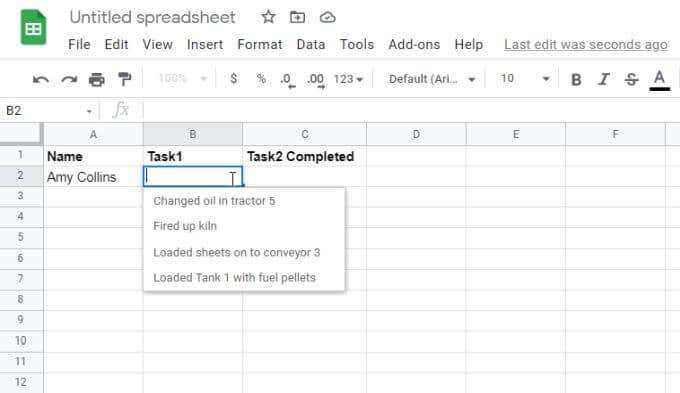
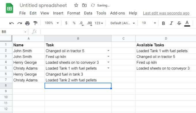
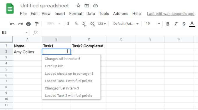
One more useful way to use Google Sheets dropdown lists is to pass information between sheets. You can also use this technique to relay information between people.For example, if you have an original sheet that contains a list of tasks completed by one team, you can base a second spreadsheet on those completed tasks.You may or may not want to create that first list based on the same dynamic dropdown lists as described in the last section.Either way, select the cell on the sheet you want to send the completed tasks to as another dropdown list, and open the validation window as described in the last section. When you select the data range, switch to this source task spreadsheet and select the entire column of tasks (including blank cells).Now, on the destination spreadsheet, you’ll see that the data from the tasks column is pulled in. This means your second team can perform their own project tasks based on completed tasks from the first team.The first team can continue adding newly completed tasks to the original source spreadsheet.Since you included the blank cells in the source range, those new unique tasks will appear in the second team’s dropdown list. Keep in mind that only unique tasks will appear in the second dropdown list. It isn’t the best way to pass specific row items from the source, but it is a great way for a second team to see all unique items added to a spreadsheet by other people.
How Will You Use Google Sheets Dropdown Lists?
As you can see, Google Sheets offers many ways you can pull information from other cells to fill out dropdown lists. Or, if your data entry needs are fairly simple, you can stick to manually entering in dropdown list items separated by commas. Either way, you should be able to make data entry for any of your spreadsheets as easy and simple as possible.
